Capabilities of Bond Testing: Pitch-Catch, Mechanical Impedance Analysis, and Resonance Bond Testing

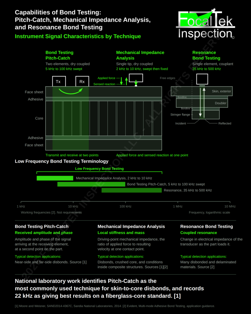
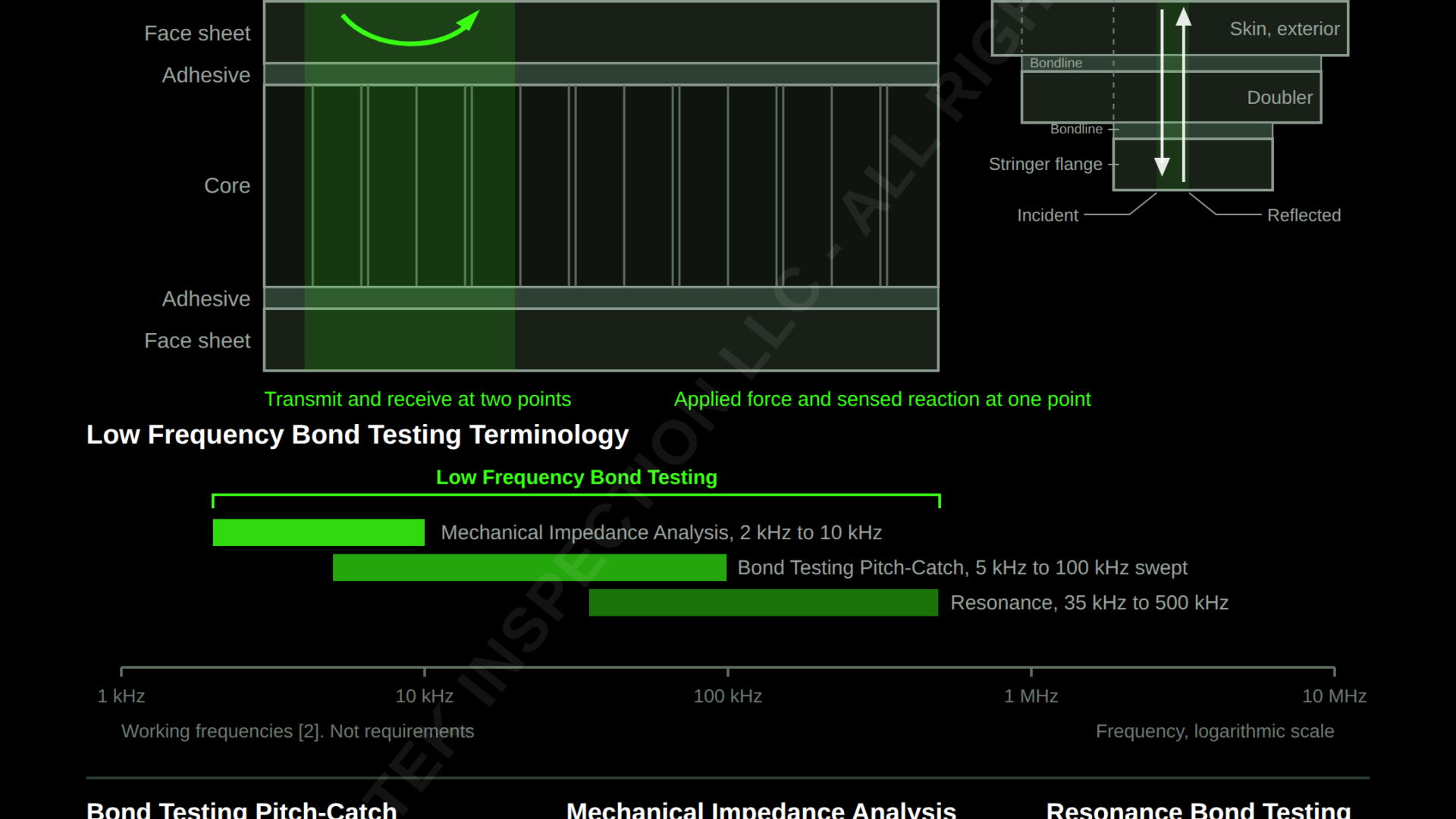
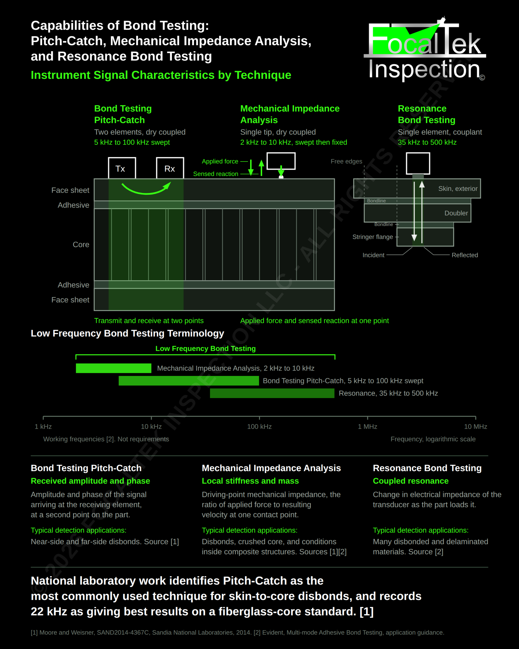
Figure 1. Instrument Signal Characteristics by Technique, with working frequencies. Sources as listed on the figure and in the article.

Scope

This article addresses the capabilities of the different Bond Testing techniques and the instrument signal characteristics that are used in each of the techniques, as well as the frequency and probe variables that are specific to each technique.

One Condition, Three Reports

Three technicians examine the same location on the same bonded honeycomb panel on the same morning. Each is qualified and certified. Each works to a written procedure. Each uses a different one of the three Bond Testing techniques.

The technician working Bond Testing Pitch-Catch watches amplitude rise and phase shift as the probe crosses the area. A boundary goes on the skin, and the report records a skin-to-core disbond.

The technician working Mechanical Impedance Analysis (MIA) watches the impedance plane move as local stiffness falls beneath the tip. A boundary goes on the skin. It does not match the first one.

The technician working Resonance Bond Testing watches the loading on the transducer change across part of that area and hold steady across the rest. The report records a separation, and records which bondline it sits on.

Three reports. Three boundaries. One panel.

The reflex is to ask which technician got it right, and to treat the disagreement as something to be settled by a repeat examination or a fourth opinion. The disagreement is not an error. The three technicians measured three different physical quantities, and each reported what the instrument in hand read. Pitch-Catch reads amplitude and phase arriving at a second element on the part. MIA reads the ratio of applied force to resulting velocity at one point. Resonance reads the change in the transducer’s own electrical impedance as the part loads it. The contact footprints differ as well, so the three are not integrating over the same area of skin.

Three different inspections of one structure, using three different techniques, are likely to produce more than one indication boundary. What the three reports are worth to the engineer who receives them depends on whether that is understood when the work is planned, or discovered afterward.

The scenario above is hypothetical.

1. Instrument Signal Characteristics

1.1 Common Elastic Basis

What is a bond test instrument actually sensitive to, and what is it inferring from that sensitivity?

Start with what a bondline does when it is intact. It carries load across an interface, and it carries sound across the same interface, because those are the same continuity. Acoustic impedance is density times velocity, and velocity follows from stiffness and density, so a change in how the stack holds together is a change in how it carries sound. Separate the interface and both go at once. That single fact is what all three techniques are built on, and it also bounds what any of them can establish: each measures a mechanical or acoustic consequence of the bond, and adhesion is inferred from that consequence. The inference is examined in section 7.

Which consequence each technique measures, and at which point on the part, is what separates the three. Technique selection is made there, before the instrument is picked up, and it remains a judgment for qualified and certified personnel against the construction in hand.

1.2 Where the Probe Touches and Where It Listens

Every measurement here starts with a probe touching a surface. What separates the three techniques is how many places they touch, and where they listen.

Bond Testing Pitch-Catch

Contact points on the part: two, at fixed separation.

Where the response is sensed: at the receiving element, a second point on the part.

Mechanical Impedance Analysis

Contact points on the part: one.

Where the response is sensed: at the same point that is driven.

Resonance Bond Testing

Contact points on the part: one.

Where the response is sensed: on the same element that drives.

Drive a point and read the motion at that same point, and the quantity measured is what that one spot pushes back with. This is a driving-point measurement, and it is a property of the structure directly beneath the tip. Move the receiver to a second point and the quantity changes: what is now measured is what reached the second point from the first, which is a transfer measurement and a property of the path between them. MIA and Resonance Bond Testing are built the first way. Pitch-Catch is built the second way deliberately, because the path between the two tips is what crosses a disbond.

For the examination that difference decides what a result means. A driving-point technique reports on the material under one tip, so the tip position is the indication position. A transfer technique reports on a line, so an indication belongs somewhere along that line and the probe orientation is part of the record. Unless the technique states the scan directions used, coverage on a transfer technique is not reproducible by the next technician.

1.3 Material Velocities and the Mode Each Technique Works In

The velocities quoted below are taken from a published material sound velocity table [4]: graphite/epoxy composite 0.1200 in./µs, fiberglass 0.1080 in./µs, aluminum 0.2490 in./µs. Composite velocity varies with layup, fiber volume fraction, fiber orientation, resin system and cure parameters, so these are representative published figures and not properties of any particular part.

Those are bulk longitudinal velocities, of the kind used for ultrasonic thickness measurement, and they describe a longitudinal wave travelling through the thickness. They are not a single velocity that serves all three techniques, because the three techniques do not work in the same mode. Which mode a technique works in decides whether this table is its velocity or only a reference for scale.

Bond Testing Pitch-Catch

Mode it works in: the first asymmetrical Lamb mode, flexural, in the near-surface layer [2].

What the velocity table is for it: not its velocity. A flexural wave runs on the bending stiffness of the layer in its own plane and on its mass per unit area, and that table carries neither. It is also dispersive, meaning its velocity changes with frequency, so a single table entry misrepresents it. Quoted here only to set the frequency regime.

Mechanical Impedance Analysis

Mode it works in: no propagating wave at the working frequency. A driving-point stiffness at one contact.

What the velocity table is for it: not a velocity of the technique at all. Quoted only to show that the whole stack is a small fraction of one wavelength, so the stack moves as one piece instead of carrying a wave. That is what makes the spring model in 2.2 available.

Resonance Bond Testing

Mode it works in: the probe runs at its own resonance and reads the acoustic load the part returns. The idealized part-side model is a through-thickness standing wave, and 2.3.6 sets out a second candidate, a flexural resonance of the separated region.

What the velocity table is for it: the correct velocity for the through-thickness model, which is a longitudinal wave through the thickness, so the thicknesses computed in 2.3.4 follow from it directly. It does not serve the flexural candidate, which needs in-plane constants.

The distinction carries a further consequence for the composite cases. A laminate is anisotropic, and the published figure is the through-thickness velocity. The flexural behavior that governs Pitch-Catch depends on the in-plane elastic constants instead, which no consulted source supplies. That is why a through-thickness resonance is computed for Resonance Bond Testing while no flexural wavelength is computed for Pitch-Catch, and why the flexural resonance in 2.3.6 is carried only as a scaling from published measurement.

1.4 Bond Testing Pitch-Catch

1.4.1 Configuration

Two elements in a single probe housing at fixed separation, dry coupled to the surface. One element transmits and one receives. Dry coupled means the contact is made by the tip material against the surface under hand pressure, with no liquid in the path. Tip condition and hand pressure are therefore technique variables in their own right. A worn, flattened or contaminated tip and a lighter hold both change the contact, and the reading moves with the part unchanged.

1.4.2 Operating Frequency

Unless the governing technique specifies otherwise, the working range for the swept mode runs 5 kHz to 100 kHz, with a selectable bandpass of 0 kHz to 35 kHz available for “each pitch-catch method” to filter noise from probe movement [2]. The instrument the mode runs on reaches further: 1 kHz to 50 kHz for radio frequency and impulse, and 5 kHz to 100 kHz swept [3]. The swept figures coincide. A second manufacturer publishes no per-mode figure at all, giving one instrument span of 250 Hz to 1.5 MHz, and stating that frequency is probe and setup specific [7].

That last point is the one that matters at the part. Frequency on this technique belongs to the probe and to the setup established on the reference standard, and it is recorded as a technique input per section 8(a).

1.4.3 Instrument Signal Characteristics

Amplitude and phase of the signal arriving at the receiving element. Both are read, and both matter, because they move for different reasons: amplitude responds to how much energy leaked away into the structure below, and phase responds to how fast the wave crossed the gap between the tips. 2.1 works both mechanisms. An examination set up on amplitude alone still functions, but it carries only half of what the probe is returning, and that choice belongs in the technique rather than in the operator’s habit.

1.4.4 Reported Capability

Skin-to-core disbonds are the condition this technique is most often pointed at, and national laboratory work records Pitch-Catch as “of the most commonly used test method for skin to core disbonds” [1]. The same work found 22 kHz gave the best results for both near-side and far-side disbond [1].

Read the conditions on that figure before carrying it anywhere. It was obtained on one reference standard, a fiberglass-core article identified as CHRS-2-6 to ARP 5606 Composite Honeycomb NDI Reference Standards, on one core material [1]. It establishes that a frequency in that region worked on that construction. Extending it to a graphite/epoxy skin over an aluminum core would go past the evidence, and the frequency for any given part is found on a standard built to that part’s construction.

1.4.5 Wavelength Scale

The published velocity table [4] gives bulk longitudinal velocities. Across the published 5 kHz to 100 kHz working range [2], those velocities correspond to bulk longitudinal wavelengths of 24 in. down to 1.2 in. in graphite/epoxy, 21.6 in. down to 1.08 in. in fiberglass, and 49.8 in. down to 2.49 in. in aluminum. Those figures establish the frequency regime. They are not the wavelength this technique propagates, which is the first asymmetrical Lamb mode in the near-surface layer, dispersive and travelling well below the bulk longitudinal velocity. That wavelength is shorter than the figures above and is not computed here, because no consulted source supplies the elastic constants and areal density the flexural relation requires.

1.5 Mechanical Impedance Analysis

1.5.1 Configuration

A single tip in dry contact with the surface. The tip is driven and the reaction developed at that contact is sensed at the same point. The quality of that dry contact is part of the measurement rather than a condition around it: 2.2.2 shows the response scales on the ratio of contact stiffness to disbond stiffness, so tip condition and the pressure held are inside the result.

1.5.2 Operating Frequency

The drive frequency is swept through 2 kHz to 10 kHz at setup to establish the optimum test frequency, and testing is then performed at that fixed frequency [2]. The consulted source does not define what makes a frequency optimum. In practice it is the frequency at which the bonded and disbonded conditions on the reference standard sit furthest apart on the impedance plane, and 2.2.6 gives the reason such a frequency exists and why it cannot be calculated in advance. The frequency selected is a technique input and is recorded, per section 8(a). The instrument specification for the same manufacturer’s bond tester gives a wider span for the mode, 2 kHz to 50 kHz [3], so the working range and the instrument range are not the same figure.

1.5.3 Tip Diameters Offered

MIA probes are published with tip diameters of 12.7 mm (0.5 in.) and 6.35 mm (0.25 in.) [6]. The tip diameter sets the contact footprint, which is the area over which the reaction is developed.

1.5.4 Instrument Signal Characteristics

Driving-point mechanical impedance, which is the ratio of applied force to the resulting velocity at the contact, read in magnitude and phase. The quantity is complex by definition: a reactive part, which stores energy and comes from stiffness and mass, and a resistive part, which absorbs it and comes from damping. Those two parts move independently, which is why the display is a plane and not a meter, and why a change in one can be told from a change in the other. 2.2.6 works the relation.

1.5.5 Where the Return Is Measured

The return arrives at the same tip that applied the force. A driving-point impedance is defined at one point, so nothing is sent to a second point on the part and nothing needs to be.

1.5.6 Reported Capability

Disbonds and crushed core are where this technique is reported to perform, in national laboratory work that records it “works well to detect disbonds and crushed core conditions” [1] and in manufacturer application guidance that adds “bond defects on the inside wall of a composite structure” [2]. Neither source states a detection capability as a size at a depth in a named construction, so each statement transfers to a part only on demonstration on a standard carrying that condition.

1.5.7 Wavelength Scale

MIA reads a driving-point stiffness at one contact, so no wave propagates along the part at the working frequency. The published velocity table [4] is useful only for scale: across the published 2 kHz to 10 kHz working range [2], bulk longitudinal wavelengths run 12 in. to 60 in. in graphite/epoxy and 25 in. to 125 in. in aluminum, so a stack 0.75 in. thick is a small fraction of one wavelength at every frequency in that range. The whole 0.75 in. stack moves together, in step, like a weight on the end of a spring. The tip is loaded by a stiffness, and the response is a stiffness reading, with no echo and no time of flight to gate on. That is what makes the spring model in 2.2 available.

1.6 Resonance Bond Testing

1.6.1 Configuration

A single resonant element coupled to the part through a liquid couplant. The instrument reads the change in that element’s own electrical impedance as the part loads it, so the one element both drives and senses.

1.6.2 Operating Frequency

Working frequencies for this mode run 35 kHz to 500 kHz, with the higher frequencies going to thinner or metallic layers [2]. The instrument itself reaches lower than that, 1 kHz to 500 kHz for the mode [3]. Sending the higher frequencies to thinner or metallic layers is a consequence of the physics rather than a manufacturer preference, and 2.3.5 shows both halves of it falling directly out of the thickness resonance relation. That is worth knowing before a probe is chosen for a construction nobody has run before.

1.6.3 Probe Frequencies Offered

Resonance probes are published at six nominal frequencies, each with a published tolerance: 35, 65, 110, 165, 250 and 330 kHz [5]. The lowest offered, 35 kHz, is the lower bound the same manufacturer’s application guidance gives for the technique [2].

1.6.4 Instrument Signal Characteristics

Change in the electrical impedance of the transducer as the part loads it, read in magnitude and phase. The instrument measures at its own terminals, so what reaches the display has already passed through the couplant film and the transducer before it represents anything about the part. 2.3 works that chain, and 2.3.2 gives the consequence for what the technician controls by hand.

1.6.5 Reported Capability

Many disbonded and delaminated materials fall to this technique, and “in many cases, the disbond depth can be related to the rotation of the signal phase” [2]. That second point separates Resonance from the other two, since neither Pitch-Catch nor MIA is reported as returning depth. The hedge in the source is real and is kept here: the relation between phase and depth is established on a reference standard carrying separations at known depths, and is not read off the instrument on an unknown construction.

1.6.6 Area Covered per Reading

Near field length and beam spread are computed from the probe face diameter and the frequency, and no resonance probe face or element diameter was located in published form from either manufacturer. Evident publishes resonance probe part numbers, nominal frequencies with tolerances and case diameters, but no face or element diameter [5]; no NDT Systems publication consulted carries per-probe frequency or dimensional data for its Bond Test probes [7][8]. Neither is therefore computed here.

The area a probe covers depends on its face diameter, not on its frequency alone. A technique sheet naming only a frequency has therefore not said how much of the part each reading covers. Two 110 kHz probes with different faces read different amounts of skin per position, and a disbond small against one face can be averaged away while the other finds it. Record the probe part number and, where a face or tip dimension is published, record that too, which is what section 8(b) asks for.

1.6.7 Standing Wave

In the classical thickness resonance condition, the stack resonates where its thickness works out to a whole number of half wavelengths. The antinodes sit at the surfaces, where the material is free to move. Application material for the resonance mode words the condition differently, as odd number multiples of the acoustic wavelength in the plate [2]. The two enumerations do not describe the same series. The discrepancy is taken up in 2.3.3. Computed thicknesses are reported on the half wavelength basis.

2. Physical Basis of the Three Techniques

A bondline that has separated no longer transfers shear and normal traction across the interface, so the layers above it stop acting as one section and start acting as two. Every quantity that depends on section behavior moves: the bending stiffness of the near-surface layer, the stiffness the surface presents to a probe pressed against it, and the acoustic load the part presents to a transducer coupled to it. The three techniques are three ways of reading that one change.

2.1 Pitch-Catch: Flexural Rigidity of the Near-Surface Layer

2.1.1 What Travels Between the Tips

A Pitch-Catch probe puts neither a beam driven down through the skin nor a pulse returning from a back surface into the part. Until the mode is named, none of the setup decisions that follow it can be justified.

The transmitting tip bends the skin. That bend travels away in the plane of the skin as a plate wave, and the receiving tip, held at a fixed separation in the same housing, detects its arrival. The mode carrying most of that energy is the first asymmetrical Lamb mode [2]. Asymmetrical describes the motion: both faces of the layer displace in the same direction at the same instant, so the layer flexes instead of compressing through its thickness. It is the flexural mode, and everything that follows turns on that one fact, because a flexural wave runs on bending stiffness and mass per unit area and not on the bulk velocity of the material. At wavelengths long compared with the layer thickness it obeys classical thin-plate flexure, and that equation is worth working, because it is where the size of the disbond signal comes from.

2.1.2 The Equation Behind the Flexural Wave

Transverse displacement of a thin plate in flexure obeys

D ∂⁴w/∂x⁴ + m ∂²w/∂t² = 0,   with   D = E h³ / [12 (1 – ν²)]

where:

●       D = flexural rigidity of the plate, force times length

●       w = transverse displacement of the plate, length

●       x = distance along the plate in the direction of propagation, length

●       t = time

●       m = mass per unit area of the plate: the mass sitting under one unit of surface, which is density times thickness. Not the total mass of the panel

●       E = elastic modulus in the plane of the plate, force per unit area

●       ν = Poisson’s ratio, dimensionless

●       h = plate thickness, length

Put a travelling wave into that equation, one of wavenumber k running at angular frequency ω, and the derivatives collapse to a single relation between the two, D k⁴ = m ω², so

k = (m ω² / D)^(1/4)   and   c_f = ω / k = ω^(1/2) (D / m)^(1/4)

where:

●       k = wavenumber, which is 2π divided by the wavelength. It counts how many wave cycles fit in a given length, so a larger k means a shorter wave. Radians per unit length

●       ω = angular frequency: the frequency set on the instrument, multiplied by 2π. Radians per unit time

●       c_f = flexural phase velocity, or how fast one point on the wave travels along the plate. Length per unit time. This is not the bulk longitudinal velocity published at 1.3

●       D and m are as defined above

The flexural mode is dispersive, meaning its velocity is not one number but changes with frequency. Flexural phase velocity c_f rises as the square root of frequency, so doubling the frequency shortens the wavelength by a factor of 1.41 rather than by half. Across the published 5 kHz to 100 kHz swept range the frequency changes by a factor of 20 while the wavelength changes by a factor of about 4.5. At the probe that means the tip separation built into the housing is a different number of wavelengths at the bottom of the sweep than at the top, so a swept response is the sum of many tip-spacing-to-wavelength relationships and not one. It also means a setup established in one frequency band is re-established on the standard rather than moved to another band by calculation.

2.1.3 What the Bondline Does to Stiffness

Over a disbond the near-surface face sheet bends alone, and its rigidity is the plate value above with h equal to the face sheet thickness. Over a bonded region the face sheet is the outer fiber of a sandwich section, and standard sandwich theory gives the rigidity of two thin faces separated by a core as

D_sandwich = E h d² / [2 (1 – ν²)]

where:

●       D_sandwich = flexural rigidity of the bonded sandwich section, force times length

●       d = distance between the mid-planes of the two face sheets, length

●       E, h and ν are as defined in 2.1.2, with h the face sheet thickness

Dividing one by the other, E and ν cancel and the ratio is purely geometric:

D_sandwich / D_face = 6 (d / h)²

where:

●       D_face = flexural rigidity of one face sheet bending alone, force times length

●       the ratio is dimensionless, and E and ν have divided out

2.1.4 Computed Rigidity Ratio

For a 0.040 in. face sheet on a 0.75 in. core, d is 0.790 in. and the ratio is 2,340 to 1. For a 0.030 in. face sheet on a 0.50 in. core, d is 0.530 in. and the ratio is 1,873 to 1. The bonded section is on the order of two thousand times stiffer in bending than the same face sheet acting alone. That is the size of the change Pitch-Catch is looking for at a disbond: not a few percent, but a different structure under the probe. The ratio holds for any face sheet material because the material terms divided out, so the same 0.040 in. skin on the same 0.75 in. core gives 2,340 to 1 whether the skin is graphite/epoxy, fiberglass or aluminum.

2.1.5 Consequence for the Signal

Flexural phase velocity goes as the fourth root of rigidity over areal mass, so a rigidity ratio of 2,340 to 1 would correspond to a velocity ratio of 6.96 to 1 if the two sections carried the same mass per unit area. They do not. The bonded section carries a second face sheet, which doubles the face sheet mass on its own and brings the figure to 5.85 to 1 before any core mass is counted, and the core mass lowers it further.

That figure is the arithmetic of static bending and is not a prediction of the working velocity ratio. Standard sandwich panel treatments set out three regimes: pure bending of the whole section at low frequency, a core shear controlled regime above a transition frequency, and face sheet bending at high frequency. The working band is expected to sit in the core shear controlled regime. No consulted source gives the transition frequency for any construction, so there is no way to confirm that for a given part, and the static bending relation is therefore not taken to set the wave speed here.

What the geometry does establish is the mechanism and the wavelength direction. The bonded section is stiffer in bending than the separated face sheet by three orders of magnitude in static terms, and guided wave measurements on honeycomb sandwich over 15 kHz to 50 kHz report that a debonded skin carries a significantly larger wavenumber than the intact sandwich beside it, which at a given frequency is a shorter wavelength and a lower phase velocity, and that the group velocity in the debonded skin is higher than in the intact sandwich [13]. The group velocity result is consistent with a core shear limited sandwich wave, and is the opposite of what the static rigidity ratio alone would suggest. The phase velocity result runs the direction the static ratio predicts. The phase of the signal arriving at the receiving element moves with the wavelength change. That is the physical reason the instrument reads phase, and the reason probe tip spacing is a technique input. Across a probe of fixed tip separation, the phase difference between the bonded path and the separated path can exceed one full cycle. When it does, the phase wraps: 360 degrees of rotation plots in the same place as zero. A large or deep separation can therefore read as sound structure. The check belongs on the standard. Walk the probe across every condition the standard carries and confirm the phase runs one way without doubling back. Where two different conditions land on the same phase angle, that setup cannot separate them, and either the frequency or the probe has to change.

2.1.6 The Separate Amplitude Mechanism

Amplitude moves for a second and separate reason, and the two mechanisms can be defeated independently. Over bonded structure a portion of the energy is attenuated by what sits below the examination surface; over a disbond the wave travels between the transmitting and receiving elements with very little attenuation or damping from the structure beneath [2]. A face sheet coupled to a core radiates energy into the core as it bends. A face sheet separated from the core radiates far less, so more of the energy stays in the plate and arrives at the receiving element. Loss is reduced rather than eliminated, since the separated region still radiates into air, leaks across the boundary of the separation, and loses energy to damping in the resin. Amplitude and phase therefore respond to separate mechanisms, and an examination set up on amplitude alone does not carry the phase response described above.

2.1.7 Limits of the Flexural Treatment

The modulus and Poisson’s ratio of any particular face sheet, and the areal density of any particular core, are not supplied by any consulted source. No absolute flexural velocity or wavelength in a bonded sandwich is computed. The geometric rigidity ratio stands without them; an absolute velocity does not.

2.2 Mechanical Impedance Analysis: A Spring Over the Structure

2.2.1 The Published Spring Model and a Discrepancy

The loading on the receive element at the bottom of the probe cone is set by the stiffness of the sample beneath it, and that stiffness falls from very high to low between bonded and disbonded structure [2]. The same guidance sets out the spring model developed by P. Cawley, in which over a disbond the spring stiffness is the contact stiffness of the probe in relation to the defect stiffness, and over a well bonded composite the spring stiffness is only the contact stiffness [2].

Cawley’s own published statement of the model puts the elements in a different order, and the difference matters. The published work models a disbond or delamination as a spring beneath which lies the undamaged structure, with the spring stiffness infinite where no defect is present, and reports that the technique is most sensitive where the defect is close to the surface and the base structure is relatively stiff, and that the limiting factor on sensitivity is the stiffness of the dry point contact between the transducer and the structure [12]. The series pair in the published model is therefore the defect spring and the structure beneath it, with the contact stiffness setting the sensitivity limit rather than forming one half of the pair.

2.2.2 The Two Springs in Series

The relation worked below takes the two compliances in series as the probe contact and the disbond, which is the application guidance rendering [2]. It is the form the instrument documentation states, and it is not Cawley’s published pair. Stack two springs end to end and the pair gives more under the same push than either spring alone. In that arrangement it is the compliances that add, compliance being the give of a spring, one divided by its stiffness. So

1 / k_eff = 1 / k_c + 1 / k_d,   and therefore   k_eff / k_c = 1 / (1 + k_c / k_d)

where:

●       k_eff = effective stiffness presented to the probe tip, force per unit length

●       k_c = contact stiffness of the probe tip on the surface, force per unit length

●       k_d = stiffness of the disbond, force per unit length, taken as infinite where no separation is present

The response depends on the ratio of the two stiffnesses and not on the disbond stiffness by itself. If the contact stiffness is small enough compared with the disbond stiffness, a disbond of any size and any compliance produces no change at all in what the probe reads. That is what a poor contact looks like in service: a worn tip, a contaminated or painted surface, a tip held at an angle, or lighter hand pressure than was used on the standard. The screen sits still over a real disbond and looks the same as sound structure, which is why the transfer check in section 6 is performed on the part itself.

2.2.3 Computed Stiffness Ratio

Taking the ratio k_c/k_d across two decades: at 0.1 the effective stiffness falls by 9 percent; at 0.5 it falls by 33 percent; at 1.0 it falls by 50 percent; at 5.0 it falls by 83 percent; at 10 it falls by 91 percent. The change grows steadily as the ratio grows, with no step and no threshold anywhere in those numbers. That is what appears at the probe: scanning a tip across the edge of a disbond, the spot drifts across the impedance plane instead of jumping, and the screen gives no mark for the edge. Where the boundary goes is a judgment about where the drift started, against the alarm or box set on the reference standard. Two technicians working the same disbond to the same procedure can mark two boundaries a quarter inch apart and both be reading their instruments correctly.

2.2.4 Consequence for Reference Standards

Defect samples made from polytetrafluoroethylene inserts may not be readily detected by the MIA technique, because the inserts stiffen the simulated disbond [2]. The series model says the same thing in numbers. Polytetrafluoroethylene is stiffer than an air gap, so an insert raises k_d, and raising k_d lowers the ratio k_c/k_d. Run that back through 2.2.3: a ratio falling from 1.0 to 0.1 takes the response from a 50 percent fall in effective stiffness to a 9 percent fall. A standard built correctly to its drawing, with the insert at the right size and the right depth, can therefore fail to represent the condition it was built for. That is a physical result about the technique, not a workmanship problem with the standard.

2.2.5 Consequence for Probe Tip Diameter

The contact stiffness of a rigid flat punch on an elastic half space is proportional to the contact radius rather than to the contact area. Applied to the published tip diameters of 0.5 in. and 0.25 in. [6], that relation would place the two tips a factor of two apart in contact stiffness, and therefore a factor of two apart in the ratio k_c/k_d for the same disbond.

The half space condition is not satisfied on a thin face sheet. The contact radius at both published tip sizes is several times the thickness of a typical face sheet, so the backing and the local bending of the plate both feed into what the tip reads. The flat punch relation therefore describes a textbook contact on a thick block and not the contact a tip makes on a 0.040 in. skin, so the factor of two is not a number to design to. What does carry over is the direction. The larger tip presents the higher contact stiffness. Higher contact stiffness means a higher k_c/k_d ratio, and 2.2.3 shows a higher ratio gives a larger fractional change for the same disbond. The 0.5 in. tip is therefore the more sensitive of the two while averaging over four times the area, and the 0.25 in. tip resolves a smaller disbond in extent while giving less response to it. A tip change moves both at once, so it is a setup change: the standard is re-run and the response re-established.

2.2.6 Basis for the Impedance Plane Display

Driving-point mechanical impedance is the ratio of applied force to resulting velocity at the driven point. For a lumped contact,

Z(ω) = R + j [ ω m_e – k_eff / ω ],   magnitude minimum at   ω₀ = (k_eff / m_e)^(1/2)

where:

●       Z(ω) = driving-point mechanical impedance at the contact, force per unit velocity

●       R = mechanical resistance: the part of the load that absorbs energy instead of storing it, which is the damping. Force per unit velocity

●       j = the imaginary unit, the same j as in electrical impedance. It marks the term sitting 90 degrees out of phase with the resistive term, which is why this display is a plane and not a meter

●       m_e = effective mass: how much material actually moves with the tip, treated as one block on the end of the spring. Distinct from the mass per unit area m of 2.1.2, and from the total mass of the part

●       ω₀ = angular frequency at which the magnitude of Z is a minimum

●       ω and k_eff are as defined above

Below that frequency the term in brackets is negative and the contact is stiffness controlled. Above it the term is positive and the contact is mass controlled. Sound structure under the tip gives one ω₀. A disbond under the tip lowers k_eff and gives a lower ω₀. That is what the setup sweep in 1.5.2 is doing. Where the frequency fixed at setup sits between those two, crossing onto the disbond carries the contact through its resonance and both magnitude and phase swing hard. Where the frequency is fixed above the bonded ω₀ instead, the disbond only pushes the contact further onto the mass controlled side. The reading still moves, but far less, and the shift is spent chasing a small signal that could have been made large at setup. This is the physical reason the optimum frequency is found by sweeping on the standard and is not calculated. A separation also changes the participating mass, because more of the skin moves, so the shift in ω₀ is not attributable to the stiffness term alone. Magnitude and phase are separate readings of the same event, and the instrument displays them as a plane because a single amplitude cannot distinguish a stiffness fall from a damping rise.

The two relations above describe different regimes and are not interchangeable. The series stiffness relation above is static and carries no frequency; it describes the contact well below resonance. The impedance relation is dynamic. Where the instrument operates close to resonance, the percentages computed above describe the change in the stiffness term and not the change in the instrument reading.

2.2.7 Limits of the Spring Model

Nothing in the consulted set supplies a value for the contact stiffness of any probe, the stiffness of any disbond, the effective mass, or the damping. The model establishes the form of the response and the variables that govern it. It does not predict the size of the response on any part.

2.3 Resonance Bond Testing: A Loaded Transducer

2.3.1 Why the Transducer Reads the Part

A resonance probe has no separate receiver. The same element drives the part and reports on it, and it does so through its own electrical terminals: the measured electrical impedance of the transducer is affected by the acoustic impedance of the sample beneath it, and that acoustic impedance is altered by any lack of bonding [2]. The instrument is reading an electrical quantity and inferring a mechanical one, which makes the inference chain longer here than in either of the other two techniques. The same guidance further states that the instrument automatically selects the resonance frequency of the transducer in air by sweeping a frequency range and locating the phase null, and then operates at that frequency [2].

2.3.2 What the Operating Point Fixes

The starting frequency belongs to the probe, not to the part. The examination starts from a frequency found with the probe held in air, and the part then loads that resonator. The instrument then operates at that frequency in the run modes [2], so the drive is fixed while the load is not. What appears at the transducer’s electrical terminals is not the crystal alone. It is the crystal, the couplant film and the part behaving as one system, and 2.5 gives that as the limit of treating this as a single resonator. The practical weight falls on the couplant film, because it is the one element in that stack the technician sets by hand and resets at every position. Couplant type, film thickness and the pressure held on the probe all sit inside the measurement. Change any of them between the standard and the part, or let any of them drift across a scan, and the reading moves with the part unchanged. No consulted source quantifies that sensitivity, so it is not computed here. The working consequence is that whatever couplant and hand pressure produced the setup on the standard are what has to be reproduced on the part, and the transfer check in section 6 is where that is confirmed. The probe frequency remains a technique input fixed at probe selection, which is why the technique is supplied as a set of nominal probe frequencies.

2.3.3 The Part-Side Condition and a Discrepancy

A disbond acts as a thin plate that vibrates, generating a standing wave when the thickness equals odd number multiples of the length of the acoustic wave in the plate [2]. The classical thickness resonance condition for a plate free on both faces is a thickness equal to an integer number of half wavelengths:

t = n c_L / (2 f),   equivalently   f_n = n c_L / (2 t)

where:

●       t = thickness of the resonating layer, length. In this relation t denotes thickness, not time as in 2.1.2

●       n = harmonic number: which resonance is being counted. 1 is the fundamental, 2 the next one up, 3 the one above that

●       c_L = bulk longitudinal velocity through the thickness, length per unit time. This is the velocity published at 1.3, and it is not the flexural phase velocity c_f of 2.1.2

●       f = frequency

●       f_n = frequency of the nth harmonic

The two do not give the same answers. Half wavelengths put resonances at 0.5, 1.0 and 1.5 wavelengths of thickness. Odd multiples of a full wavelength put them at 1, 3 and 5. The first thickness in each list is different, and so is every one after it. Odd multiples of a full wavelength is not the resonance condition for a plate under any standard pair of boundary conditions, so the published wording is not reconciled with the classical relation by a change of boundary condition. The computations below use the classical half wavelength condition and are reported on that basis. The practical consequence of the discrepancy is that a depth mapping is established on a reference standard carrying the construction present in the part, and is not taken from this calculation.

2.3.4 Computed Half-Wave Thickness

Half wavelength thickness at each published resonance probe frequency [5], computed from the published bulk longitudinal velocities [4], which are the correct velocities for a through-thickness resonance.

35 kHz: graphite/epoxy 1.71 in., fiberglass 1.54 in., aluminum 3.56 in.

65 kHz: graphite/epoxy 0.92 in., fiberglass 0.83 in., aluminum 1.92 in.

110 kHz: graphite/epoxy 0.55 in., fiberglass 0.49 in., aluminum 1.13 in.

165 kHz: graphite/epoxy 0.36 in., fiberglass 0.33 in., aluminum 0.75 in.

250 kHz: graphite/epoxy 0.24 in., fiberglass 0.22 in., aluminum 0.50 in.

330 kHz: graphite/epoxy 0.18 in., fiberglass 0.16 in., aluminum 0.38 in.

The velocities behind these numbers are representative published figures for the material classes named and are not properties of any particular part. Each line says which thickness resonates at which frequency for a bare plate with nothing bonded to either face and nothing damping it. Set any of them against a face sheet a few tens of thousandths thick and the mismatch is the point: no thickness listed is a face sheet thickness. They are no basis for selecting a probe on any construction.

2.3.5 Why Thinner and Metallic Layers Take Higher Frequencies

Frequencies of 35 kHz to 500 kHz are given as the working range for this mode, with the higher frequencies going to thinner or metallic layers [2]. Both halves of that practice fall out of the relation above, which is worth seeing worked rather than taken on trust. Thickness appears in the denominator, so a thinner layer resonates higher. Velocity appears in the numerator, so a material of higher velocity resonates higher at the same thickness, and the aluminum column sits at roughly twice the graphite/epoxy column throughout because the published aluminum velocity is roughly twice the published graphite/epoxy velocity [4].

2.3.6 Two Candidate Part-Side Resonances

Inverting the thickness relation for a face sheet acting alone in graphite/epoxy gives a fundamental of 1,500 kHz at 0.040 in., 750 kHz at 0.080 in., and 500 kHz at 0.120 in. The highest probe offered in the published kit is 330 kHz [5], so a face sheet of 0.040 in. or 0.080 in. has no through-thickness resonance reachable by any offered probe. At 0.120 in. the fundamental coincides with the 500 kHz top of the published band [2], which no offered probe reaches.

That is a result about the thickness mode alone. The published wording describes a separation as a thin plate that vibrates [2], which is a flexural resonance of the separated region rather than a through-thickness standing wave, and its frequency is set by the lateral extent of the separation as well as by the layer thickness. A flexural plate resonance drops with the square of how wide the separation is. Double the width and the resonance falls to a quarter of the frequency. Disbond size moves this number fast, and the size is not known before the disbond is found. Published modelling and measurement of local defect resonance places the fundamental of a 40 mm diameter flat-bottomed hole at 1 mm depth in aluminum at about 7.43 kHz [14]. A flat-bottomed hole is not a separation in the sense of 6, and aluminum is not a composite face sheet, so that figure supports an order of magnitude only. Scaling that published figure on the square relation: a 25 mm separation is 40/25 as narrow, so its resonance sits (40/25)² = 2.56 times higher than 7.43 kHz, which is near 19 kHz. That falls below the 35 kHz bottom of the resonance probe band, and inside the 5 kHz to 100 kHz Pitch-Catch working range instead. It sits above the 2 kHz to 10 kHz MIA working range, though within that mode’s wider instrument span. Computing it for any particular construction would require the elastic constants and areal density that no consulted source supplies, and a boundary condition at the edge of the separation that is not knowable in advance.

Taken together, the two results establish that the technique is not operating on one identifiable part-side resonance. It operates at the probe resonance and reads the acoustic load the part returns, which is the electrical impedance mechanism the guidance states [2]. Which part-side resonance contributes, and by how much, is established on a reference standard.

2.3.7 The Same Physics at 1 MHz

The same thickness resonance physics turns up an order of magnitude higher in frequency, on a different instrument, and the thickness-mode result above is what predicts where. For disbonds between an inner skin and a core, the published applications material describes a separate technique using a broad bandwidth 1 MHz probe driven by a square wave pulse, with the receiver filter tuned to the thickness of the structure and to the corresponding half wavelength, and it places that technique under conventional Ultrasonic Testing with a conventional flaw detector rather than under Bond Testing [11]. That is the same thickness resonance physics applied an order of magnitude higher in frequency, on an instrument whose frequency range reaches it.

2.3.8 Phase and Depth

In a multilayered joint the phase is related to the depth of the disbonded layer [2]. Take it as a loading effect on the transducer rather than as a resonance of the part, and the chain is short. The depth of the separation decides how much material sits above it. That material is what gives under the probe, so depth sets the compliance presented to the probe. In the thickness picture it also sets the length of the resonating layer above the separation, and so that layer’s resonant frequency. What the probe reads is how far that frequency sits from the probe’s own fixed frequency, above it or below it and by how much. Above and below give opposite signs, and that sign and size appear as the reactive part of the load in the transducer’s electrical impedance. On the screen it appears as the direction and the amount the signal rotates. Converting a phase angle to a depth is established on a reference standard carrying separations at known depths in the construction present.

2.3.9 Limits of the Resonance Treatment

No consulted source supplies the face or element diameter of any resonance probe, the electromechanical coupling coefficient or clamped capacitance of any transducer, or the acoustic impedance of any composite as a density and velocity pair. The relation above establishes which thickness resonates at which frequency. It does not establish the magnitude of the phase rotation for a given depth.

2.4 The Basis for Low Frequency Operation

2.4.1 Reasons the Band Is Low

The frequency separation set out in 3.3 has two causes, and they are different in kind.

The first is the quantity being interrogated. All three techniques read a stiffness or an impedance of the skin and core section as a whole. To measure a property of the whole section, the wavelength has to be much longer than the section is thick, or in the case of MIA there has to be no travelling wave at all. Raise the frequency until the wavelength comes down to ply scale and the section is no longer what is being measured. Individual plies and the boundaries between them are, which is conventional Ultrasonic Testing doing a different job, described in section 3.

The second is attenuation through the core. A honeycomb core attenuates and scatters strongly, which constrains examinations that must carry energy through the core thickness at megahertz frequencies, and is why consensus practice addresses those by Through Transmission Ultrasonics (TTU) rather than pulse-echo [16].

2.4.2 What the Low Frequency Case Leaves Open

The low frequency argument explains why Bond Testing sits where it does. It does not put conventional Ultrasonic Testing out of the running on bonded structure, and the published record runs the other way. The consensus practice for flat panel composites and flat sandwich core panels covers both constructions at 0.5 MHz to 20 MHz [9]. A second current practice covers composite sandwich constructions and names TTU for disbond detection where attenuation is high [16]. A published comparison on one honeycomb specimen set runs against the resonance technique [17]. All three are set out in 3.1 and 3.7.

Neither is it established that the core becomes a valid effective elastic medium at Bond Testing frequencies. Published guided wave work on honeycomb sandwich reports that representing the core by homogenized effective properties does not adequately represent elastic wave propagation in that material, and that retaining the real cell geometry gives a more accurate model [15]. No homogenization claim is made here.

2.5 Limits of the Models

Each of the three relations in 2.1 to 2.3 is a first-order model, meaning it keeps the one effect that dominates and drops everything else. Each real part is more complicated than the model that represents it. The differences below are the ones that show up at the probe, and they are why a model informs a technique and the demonstration remains on a reference standard. The disposition of any result remains with qualified and certified personnel and the cognizant engineering organization.

The flexural treatment assumes a plate thin compared with the wavelength, isotropic in the plane, with a disbond large enough that the separated face sheet behaves as a plate. A composite face sheet is orthotropic: it is stiffer along the fibers than across them, so its bending stiffness depends on which way it is being bent. At the probe that means one disbond can give two different responses depending on the direction it is crossed, and a Pitch-Catch probe carries its two tips on a fixed line, so it has a direction. The isotropic relation in 2.1.2 carries none of that. The reference standard and the scan plan have to: the standard is built in the layup present in the part, and the scan directions used on the part are the scan directions the setup was established in.

The series spring treatment assigns one stiffness to a contact that is distributed over a finite footprint, and one stiffness to a disbond whose compliance varies across its own area and falls to zero at its boundary. Neither is a single number in a real part. The consequence at the probe is that the model predicts the direction and the rough size of a change, and it does not predict where the edge of an indication falls, which is why the boundary is drawn against a response established on the standard.

The thickness resonance treatment assumes plane parallel faces and a single resonating layer. It carries none of the coupling between the transducer, the couplant film and the part, and that three element system is what actually sets the loaded resonance. A taper, a ramp, a ply drop or a change in couplant film thickness all sit outside the relation and inside the reading, which is the practical reason a resonance setup is re-established whenever the construction or the coupling changes.

None of the three predicts a detection capability. The consulted record contains one capability figure expressed as a disbond size at a stated depth, and it is specific: an adaptation of the Pitch-Catch technique using a purpose designed differential high voltage probe is published as reliably detecting a 25 mm by 25 mm disbond on the far side below 40 mm of honeycomb structure, a result stated to be referenced in commercial airline service bulletins [11]. That figure belongs to that probe on that class of structure. It is not a general capability of the technique, and no consulted source states a general one. Detection capability on a given construction is established by demonstration on a reference standard containing the condition of interest, holding constant the layer thicknesses, core type, bondline composition, probe dimension and operating frequency that the relations above identify as governing.

3. Conventional Ultrasonic Testing and Bond Testing on Bonded Structure

Conventional Ultrasonic Testing is the established method for composite laminate examination, and it is applied to bonded structure as well. A reasonable question from anyone whose composite work runs on Ultrasonic Testing is what a bond tester adds that a flaw detector does not. The answer is in the published scope of each, and in the frequency each operates at.

3.1 Scope of Conventional Ultrasonic Testing on Composites

The consensus practice covering flat panel composites and flat sandwich core panels sets out two techniques, pulse-echo and TTU, both working with a pulsed straight-beam longitudinal wave between 0.5 MHz and 20 MHz [9]. Pulse-echo needs access to one side of the specimen and TTU needs access to both [9]. The practice excludes contact angle-beam work with shear waves and surface-beam work with Lamb waves from its coverage [9]. Its scope is flat panels with parallel surfaces, it calls for a clean and smooth surface on the part being examined, and for honeycomb it directs in-service work at separation between the face sheet and the core [9].

The band and the constraints stated here are what one practice states within its own coverage. Conventional Ultrasonic Testing is applied to composite structure outside that scope and at other frequencies, and the figures here are set against the Bond Testing figures to establish the difference in regime, not to bound either method.

3.2 Where Conventional Ultrasonic Testing Runs Into Trouble

The method carries a set of limitations that the consensus guide covering nondestructive work on aerospace polymer matrix composites collects in its own summary. Among them: the method wants a reasonably flat and smooth surface; modulus, surface condition and the orientation of a separation all bear on whether it can be found; reference standards are needed and may have to be built for the work; and the method needs a liquid couplant, with the attendant risk that couplant enters faying surfaces and internal cavities or is taken up by porous material [10].

For TTU the same guide records that two transducers have to be fixtured precisely, aligned critically and moved in step, that two surfaces have to be prepared, that resolution and sensitivity are lower than for pulse-echo, and that the technique does not establish the depth of a discontinuity [10]. For contact work it records that a rough surface scatters and attenuates the energy, that the energy is not readily focused, and that sensitivity varies with how well the couplant performs [10].

3.3 The Frequency Separation

Within the scope stated above, conventional Ultrasonic Testing of composites runs from 0.5 MHz to 20 MHz [9]. The three Bond Testing techniques run from 2 kHz to 500 kHz [2]. The lower bound of the Bond Testing range sits two hundred and fifty times below the lower bound of the Ultrasonic Testing range, and the working ranges published by that manufacturer meet at 500 kHz without overlapping. The second manufacturer publishes a single instrument span of 250 Hz to 1.5 MHz [7], which reaches into the conventional band.

The two methods therefore interrogate the material at different scales. The scale ratio is not the frequency ratio, because the two do not propagate the same wave type: for a bulk wave the wavelength varies inversely with frequency, while for the dispersive flexural mode it varies as the inverse square root. In graphite/epoxy at the published bulk longitudinal velocity of 0.1200 in./µs [4], a 5 MHz longitudinal wave has a wavelength of 0.024 in. The Bond Testing techniques do not propagate a bulk longitudinal wave, so their working wavelength does not come from that table and is not stated here. What the frequency ratio establishes on its own is the scale separation.

3.4 Consequence of the Frequency Separation

A wavelength of a few thousandths of an inch resolves structure at ply scale, and pulse-echo establishes the depth of a discontinuity, which is why conventional Ultrasonic Testing is widely applied to delamination within a laminate. The resolution available is of the order of half a wavelength, so at the 0.024 in. wavelength computed above the figure is roughly 0.012 in. against a ply a few thousandths of an inch thick. Resolution at the scale of a single ply belongs to the upper part of the published band rather than the middle of it.

Operating far below that band, the Bond Testing techniques resolve nothing at ply scale. They interrogate the stack as a mechanical system, which is what a bondline is. The two are measurements of two properties at two scales, and the condition of interest decides which one carries the answer.

3.5 What Each Technique Is Used For

Skin-to-core disbonds go to Pitch-Catch more often than to anything else, on the record of national laboratory work [1]. MIA is pointed at disbonds and crushed core [1][2], and at “bond defects on the inside wall of a composite structure” [2]. Resonance covers many disbonded and delaminated materials, and in many cases relates disbond depth to the rotation of the signal phase [2].

3.6 Constraint and Configuration Compared

Each of the following is a limitation the Ultrasonic Testing literature states for itself, set against the Bond Testing configuration published for the same work.

Ultrasonic Testing constraint: the method needs a liquid couplant, with the attendant risk of couplant entering faying surfaces and internal cavities [10].

Bond Testing configuration: Pitch-Catch and MIA are dry coupled. Resonance uses a liquid couplant.

Ultrasonic Testing constraint: TTU needs access to both sides of the specimen [9][10].

Bond Testing configuration: all three techniques are applied from one surface.

Ultrasonic Testing constraint: TTU needs two transducers fixtured precisely, aligned critically and moved in step, on two prepared surfaces [10].

Bond Testing configuration: Pitch-Catch carries both elements in one housing at fixed separation. MIA and Resonance are single-element or single-tip.

Ultrasonic Testing constraint: TTU does not establish the depth of a discontinuity [10].

Bond Testing configuration: in many cases disbond depth can be related to the rotation of the signal phase [2]. Any phase to depth mapping is established on a reference standard carrying separations at known depths in the construction present.

Ultrasonic Testing constraint: a reasonably flat and smooth surface is wanted [9][10].

Bond Testing configuration: MIA is a dry contact at a published tip diameter of 0.5 in. or 0.25 in. [6]. No consulted source states a surface condition limit for the technique.

3.7 Conventional Ultrasonic Testing on Laminates, Cored Panels and Bondlines

The constraints set out above are those one practice states within its own scope, and they are not the whole of what conventional Ultrasonic Testing reaches on sandwich structure. A current consensus practice covers matrix array Ultrasonic Testing of composite sandwich constructions across 0.5 MHz to 20 MHz, and identifies TTU for the detection of disbonds in materials of high attenuation, naming honeycomb and foam cores [16]. A matrix array is a two-dimensional phased array probe, so the practice is written around Phased Array Ultrasonic Testing (PAUT) equipment rather than a single-element search unit.

The published comparison on the same specimen runs the same way. National laboratory work on Nomex honeycomb carrying engineered defects reports that a 5 MHz ultrasonic C-scan detected all three engineered defects at the laminate to honeycomb interface, the smallest of them barely, and that a 110 kHz resonance examination did not reliably detect the disbonds, detecting the epoxy filled core but reporting limitations in defining the shape and borders of that class of flaw [17].

Read across those sources, conventional Ultrasonic Testing reaches the laminate, the cored panel and the bondline alike. A laminate is within the scope of the flat panel practice, pulse-echo or TTU, 0.5 MHz to 20 MHz [9]. A panel with a core is within the scope of that practice and of the matrix array practice for composite sandwich constructions [9][16]. The bondline is reached where the condition is a separation: the flat panel practice directs in-service honeycomb work at separation between the face sheet and the core [9], the matrix array practice names TTU for disbonds where attenuation is high [16], and the comparison above found the interface disbonds with a 5 MHz C-scan [17]. TTU is the configuration named for the attenuating cases, and it brings the constraints collected in 3.2: both sides of the part have to be reachable, the two transducers have to be fixtured precisely and moved in step, resolution and sensitivity are lower than for pulse-echo, and the result does not carry depth [10].

What it reads is an acoustic contrast, which places the same boundary on it that section 7 places on the three Bond Testing techniques. A separation whose faces are apart presents that contrast. A separation whose faces remain in contact transmits sound across the interface and presents very little of it, at any frequency and in either family of techniques.

3.8 Limits of the Comparison

No consulted source states a general detection capability for any Bond Testing technique expressed as a disbond size at a stated depth in a stated construction. One specific figure is published for one purpose designed probe, and is reported in 2.5. National laboratory work does compare the two methods on one honeycomb specimen set, and is reported in 3.7. The comparison in 3.6 sets published configuration against published limitation. It is not a performance comparison, and it does not establish that a Bond Testing technique will find a condition that Ultrasonic Testing missed on any particular part. That determination is made on the construction, against a reference standard containing the condition of interest.

4. Low Frequency Bond Testing Terminology

4.1 The Frequency Figures Side by Side

Three different kinds of number get called a frequency in this field, and they are not interchangeable. A working range is where a mode is used. An instrument span is what the box can generate. A discrete probe frequency is what one probe actually runs at. Reading a working range off an instrument specification, or a probe frequency off a working range, produces a technique input that cannot be reproduced. Each line below names the technique, the kind of figure it is, and the source.

Mechanical Impedance Analysis, working range: 2 kHz to 10 kHz, swept at setup then fixed [2].

Mechanical Impedance Analysis, instrument span for the mode: 2 kHz to 50 kHz [3].

Bond Testing Pitch-Catch, working range: 5 kHz to 100 kHz swept, with a selectable bandpass of 0 kHz to 35 kHz on each Pitch-Catch method [2].

Bond Testing Pitch-Catch, instrument span for the mode: 1 kHz to 50 kHz radio frequency and impulse, 5 kHz to 100 kHz swept [3].

Resonance Bond Testing, working range: 35 kHz to 500 kHz [2].

Resonance Bond Testing, instrument span for the mode: 1 kHz to 500 kHz [3].

Resonance Bond Testing, discrete probe frequencies offered: 35, 65, 110, 165, 250 and 330 kHz [5].

All three modes, second manufacturer, one instrument span with no per-mode figure: 250 Hz to 1.5 MHz, probe and setup specific [7][8].

4.2 Instrument Span and Working Range

One manufacturer publishes both, and they differ for MIA and for the radio frequency and impulse Pitch-Catch modes. For swept Pitch-Catch the two figures coincide at 5 kHz to 100 kHz. The second manufacturer publishes only an instrument span, qualified on one of the two product pages as probe and setup specific [7].

4.3 Mode Naming Across Manufacturers

Of the three Bond Testing instruments consulted, all name the same three modes: Pitch-Catch, MIA and Resonance [2][3][7][8].

Where a written practice lists Low Frequency Bond Testing as a Bond Testing technique, along with the other three techniques, the written practice must supply the definition, because the instrument literature consulted does not name it as a mode. What an examiner qualifies a candidate against is then established by that written practice.

5. Position Encoding and the Examination Record

Return to the three technicians. Each marked a boundary on the skin. When the panel goes back into service, those grease pencil marks go with it, and what reaches the file is three descriptions of three boundaries. Whether anything more than that survives is decided before the first probe touches the part.

5.1 Manual Unencoded Presentation

An impedance plane display is specified presenting the signal as a moving point, and a strip chart streaming the outputs in real time [8].

5.2 Encoded Presentation

One imaging bond tester gives the C-scan in phase, magnitude or additive view, alongside the impedance plane display and the strip chart, with position taken from XY encoder inputs and either a manual or an automatic scanner [8]. That instrument is published as compatible with other bond testers, including the same manufacturer’s BondaScope 3100 [7][8].

Imaging is therefore a capability added to a bond tester rather than a property of a single instrument. It is analogous to adding one or more encoders to a conventional Ultrasonic Testing or PAUT instrument.

Where position is not encoded, the response and the position it belonged to exist only while the probe is on the part, and what reaches the file is a judgment expressed as a boundary and an area. Where position is encoded, each response is tied to a coordinate, so the area scanned and the position of every reading are captured at acquisition, the same area can be re-scanned and compared position to position, and the data can be used for as long as it is retained after the examination. Completeness of coverage remains governed by scan and index resolution, encoder calibration, probe footprint and the scan plan.

What is retained per position is a separate question from what is displayed. An instrument storing one processed value per position produces a record supporting review of the conclusion. An instrument storing the underlying signal per position produces a record supporting review of the measurement, because the gate, the phase and the mapping can be revisited. Saving the full signal for each position is of significant value for repeated scans at cyclic examination intervals in MRO and flight operations environments.

6. Reference Standards

A reference standard is a physical article of known construction containing a condition of known type, size and thickness. Instrument settings are established on it so that each known condition produces a defined response, and responses obtained from the part are evaluated against the reference responses.

All three techniques read a property of the stack beneath the probe, so layer thickness, core type, bondline composition and local geometry affect the response. Where the standard departs from the part in any of those, the response difference between the standard and the part no longer carries the same meaning. Where the departure is large enough, the standard no longer serves as a comparator for that part.

The condition contained in the standard is a second constraint. A flat-bottom hole presents a free surface where the acoustic impedance mismatch is close to total. A separation whose surfaces remain in contact presents a smaller mismatch, since contact transmits both load and sound across the interface. A technique standardized on one is standardized on the mechanical and acoustic contrast that one produces.

Set the technique up on the standard, then take the probe to the part and find a region there is reason to believe is sound construction. Read it. Compare that reading against the reading the standard gives for its sound condition. Record both, and record the difference. That is the transfer check, and it is what turns a later difference between standard and part into evidence rather than an assumption. No consulted source states how large a transfer difference is acceptable, so the limit and the action on exceeding it come from the written technique for the work concerned.

7. Limits of the Adhesion Inference

All three techniques measure a mechanical or acoustic consequence of the bond, and adhesion is inferred from that consequence.

A kissing bond defines the limit of the inference. Where surfaces remain in contact, the mechanical and acoustic contrast each technique relies on is absent or very small while the joint may carry little load. All three techniques can then produce a response indistinguishable from a bonded condition. That is the expected outcome where contact is maintained, and not an occasional one. The inference holds only where loss of adhesion produces loss of contact.

The kissing bond is one of the most challenging bondline discontinuities to detect. Whether it can be detected or sized at all on a given construction is established by technique development and a qualification program on representative hardware, and is not assumed. A result showing no indication establishes that the contrast each technique relies on was not present at the response threshold used. It does not establish bond strength, adhesion or load carrying capability, and it is not evidence that a kissing bond is absent.

No consulted source quantifies the boundary of the adhesion inference for any of the three techniques.

8. Documentation Required for Review

An examination result is reviewable when a second qualified and certified person can reconstruct how it was produced. The following are facts available at the time of examination and unavailable afterward:

a) the technique applied, named at technique level, with the operating frequency and instrument mode selected;

b) the instrument and probe, identified by part number, including the probe frequency, the face or tip dimension, and the probe tip spacing (Pitch-Catch technique only);

c) the reference standard used, identified by number, with its construction stated, the calibration targets, the measured parameters and target values of those parameters at the calibration targets;

d) the setup transfer verification performed on the part, with the region used and the response obtained;

e) the extent of coverage, and any area not examined, with the reason why it was not examined;

f) the presentations retained per position and the format in which the data is stored;

g) the limitations applicable to the result, including the adhesion inference boundary and any construction element not represented by the reference standard.

9. Summary

9.1 What the Figures Establish

The three techniques read three different instrument signal characteristics: amplitude and phase at a second element for Pitch-Catch, driving-point mechanical impedance for MIA, and change in transducer electrical impedance for Resonance Bond Testing.

Published working frequencies place MIA at 2 kHz to 10 kHz, swept at setup and then fixed, Pitch-Catch at 5 kHz to 100 kHz for the swept mode, and Resonance at 35 kHz to 500 kHz [2]. The instrument spans published for the same bond tester differ from the working ranges for MIA and for the radio frequency and impulse Pitch-Catch modes, and coincide for swept Pitch-Catch [3], and a second manufacturer publishes no per-mode figure at all, stating that frequency is set by the probe and the setup [7][8]. Resonance probes are offered at six discrete frequencies from 35 kHz to 330 kHz [5], and MIA probes at tip diameters of 0.5 in. and 0.25 in. [6].

Published national laboratory work identifies Pitch-Catch as the most commonly used technique for skin-to-core disbonds and records 22 kHz as giving best results for near-side and far-side disbond on a fiberglass-core reference standard [1].

Computed from a published velocity table of bulk longitudinal velocities [4]: across the published MIA working range of 2 kHz to 10 kHz the bulk longitudinal wavelength is 12 in. to 60 in. in graphite/epoxy and 25 in. to 125 in. in aluminum, so a 0.75 in. stack is a small fraction of one wavelength throughout. Those figures establish the frequency regime. They are not the wavelength any Bond Testing technique propagates, which for Pitch-Catch is the dispersive first asymmetrical Lamb mode and is not computed in this work.

9.2 Mechanism

Pitch-Catch propagates the first asymmetrical Lamb mode in the near-surface layer [2], and the bonded section is stiffer in bending than the separated face sheet by 6(d/h)², computed as 2,340 to 1 for a 0.040 in. face sheet on a 0.75 in. core. That ratio implies a static flexural velocity ratio of 5.85 to 1 once the second face sheet is counted, which is arithmetic and not a prediction: guided wave measurements report a higher group velocity in the debonded skin than in the intact sandwich [13], the reverse of the direction static rigidity alone would suggest.

MIA is modelled in the published work as a defect spring over the undamaged structure, with the dry point contact stiffness setting the sensitivity limit [12]; the application guidance renders the series pair as probe contact and disbond [2]. On either rendering the response follows a stiffness ratio and collapses when a reference standard insert stiffens the simulated separation [2].

Resonance operates at the probe resonance found in air [2] and reads the acoustic load the part returns; the published probe frequencies of 35 kHz to 330 kHz [5] correspond to half wavelength thicknesses of 1.71 in. down to 0.18 in. in graphite/epoxy, computed from the published through-thickness velocity [4], while a free 0.040 in. face sheet has its fundamental thickness resonance at 1,500 kHz, above the band. A flexural resonance of the separated region scales below the resonance probe band and into the Pitch-Catch working range [14].

9.3 What Remains Unestablished

Probe internal construction beyond the statement that the MIA receive element sits at the bottom of a cone [2]. Resonance probe face or element diameter, from either manufacturer, which is why no near field length or beam spread is computed. Elastic constants for any face sheet and areal density for any core, which is why no absolute flexural velocity is computed. The core shear transition frequency for any construction. Any quantified boundary for the adhesion inference. A general detection capability for any technique expressed as a disbond size at a stated depth in a stated construction; one specific figure is published for one purpose designed Pitch-Catch probe [11], and belongs to that probe on that class of structure.

10. The Focaltek Approach

Focaltek Inspection LLC applies these distinctions as the work itself. Technique selection is made from the construction and the expected condition, and where the condition sits inside a laminate or its depth has to be reported, conventional Ultrasonic Testing is selected for that reason and the reason is recorded. Reference standards are defined to the constructions actually present in the part, including the close-outs, splices, doubler steps and free edges a plain panel standard does not represent. Setup transfer is verified on the part in a region of known good construction and recorded, so that a response difference becomes evidence. Frequency, probe part number, face or tip dimension and tip spacing are recorded as technique inputs and reproduced in the report. The adhesion inference boundary, the kissing bond limit, and any bounded coverage are stated in the technique and repeated in the report, so the engineering organization receiving the result knows what it received.

For a bonded assembly whose damage state is unknown, send the construction detail with skin thickness and layup, adhesive system and nominal bondline thickness, core or substructure, the joint geometry, the conditions of concern, and the governing customer requirement. Technique selection and the reference standard set are defined from those before anything is scanned. Information of this kind is frequently proprietary and may be export controlled. Contact Focaltek before transmitting it, so that the appropriate non-disclosure and export control arrangements are in place.

Sources

[1] Moore, D.G. and Weisner, W., Technologies Used to Inspect Composite Materials, SAND2014-4367C, Sandia National Laboratories, 2014. Public via OSTI.

[2] Evident, Multi-mode Adhesive Bond Testing, Bond Testing application guidance.

[3] Evident, BondMaster 600 bond tester datasheet, instrument specification.

[4] Evident, Material Sound Velocities, nondestructive testing tutorial appendix.

[5] Evident, BondMaster Probe Kits, probe part numbers and resonance probe frequencies.

[6] Evident, Mechanical Impedance Analysis (MIA) Probes, probe part numbers and tip diameters.

[7] NDT Systems, BondaScope 3100 product specification.

[8] NDT Systems, BondHub II product specification.

[9] ASTM E2580-17, Standard Practice for Ultrasonic Testing of Flat Panel Composites and Sandwich Core Materials Used in Aerospace Applications. This is the edition consulted. It is superseded by ASTM E2580-24, which was not consulted.

[10] ASTM E2533-17ε1, Standard Guide for Nondestructive Testing of Polymer Matrix Composites Used in Aerospace Applications. This is the edition consulted. It is superseded by ASTM E2533-21, retitled Standard Guide for Nondestructive Examination of Polymer Matrix Composites Used in Aerospace Applications, which was not consulted.

[11] Evident, Nondestructive Bond Testing for Aircraft Composites, application page.

[12] Cawley, P., “The impedance method of non-destructive inspection”, NDT International, Vol. 17, No. 2, 1984, pp. 59 to 65.

[13] Yu, L., Tian, Z., Li, X., Zhu, R. and Huang, G., “Core-skin debonding detection in honeycomb sandwich structures through guided wave wavefield analysis”, Journal of Intelligent Material Systems and Structures, Vol. 30, No. 9, 2019.

[14] Aigbotsua, J.O., Smith, R.A., Marshall, T. and Drinkwater, B.W., “Modelling Low-Frequency Vibration and Defect Detection in Homogeneous Plate-Like Solids”, Journal of Nondestructive Evaluation, Vol. 43, Article 98, 2024.

[15] Fiborek, P. and Kudela, P., “Model-Assisted Guided-Wave-Based Approach for Disbond Detection and Size Estimation in Honeycomb Sandwich Composites”, Sensors, Vol. 21, Article 8183, 2021.

[16] ASTM E3370-22, Standard Practice for Matrix Array Ultrasonic Testing of Composites, Sandwich Core Constructions, and Metals Used in Aerospace Applications.

[17] Moore, D.G. and Nelson, C.L., Damage Assessment of Composite Honeycomb Material Using Advanced Inspection Technologies, SAND2012-5975C, Sandia National Laboratories.

Sources [2] through [6] are Evident, formerly Olympus. Sources [7] and [8] are NDT Systems. Source [1] is a national laboratory report. Sources [9], [10] and [16] are ASTM consensus standards. Sources [12] through [15] are peer reviewed literature. Sources [1] and [17] are national laboratory work; [1] is co-authored with the manufacturer of sources [2] through [6] and [11], and is not independent of them.

Applicability Notice

This article is not a procedure, technique, work instruction, written practice, standard, specification, code, contract requirement, or any other governing document, and nothing in it is a requirement. It states no acceptance criteria and establishes no basis for accepting or rejecting a part.

Nothing here supersedes, interprets, relaxes, or satisfies any obligation imposed by a governing document, a customer specification, or a purchase order. Any standard named is described only within the scope that standard states for itself, and applies to other materials, applications or use cases only where another code, specification, contract or requirement invokes it. Editions and revisions change; verify every citation against the edition in force for the work at hand.

This article is not formal training, and reading it accrues no training hours and supports no qualification or certification of personnel. Technique selection, technique qualification, procedure approval and the disposition of examination results remain with the Responsible Level 3 and the cognizant engineering organization for the work concerned.

This article is general technical discussion. It is not engineering advice, inspection advice, or a recommendation for any part, assembly, structure or program, and no engineering, inspection or consulting relationship arises from reading it. It has not been reviewed against any particular construction, material, service condition or governing requirement, and it is no substitute for a technique developed, qualified and approved for the work at hand by qualified and certified personnel. Any decision about method selection, technique selection, frequency, probe, reference standard, coverage, acceptance or the continued service of any part rests with the reader and the cognizant engineering organization. Focaltek Inspection LLC accepts no liability for any action taken or not taken in reliance on this article.

Frequency figures, probe data, material velocities and reported capabilities are as published by the sources cited and have not been verified by measurement. Values computed here follow from those published figures on the stated assumptions, using the first-order models identified in the text, and illustrate the physical relations discussed. They are not properties of any part, they establish no detection capability, and they are no basis for selecting a frequency, a probe, a reference standard or an examination interval. No consulted source states a general detection capability for any Bond Testing technique as a disbond size at a stated depth in a stated construction, and none is stated here.

Section 10 describes Focaltek Inspection LLC’s general approach to this class of work. It is not an offer, a quotation, a warranty or a term of any contract, and it does not state that any described activity has been performed on any particular program. Services are performed only within Focaltek’s certified method and technique scope, under a written agreement and an approved technique defining the scope, the equipment, the personnel qualification, the reference standards and the deliverables for the work concerned. No warranty of any kind, express or implied, including any implied warranty of merchantability or fitness for a particular purpose, is given in respect of this article or its content.

Product names identified in this article are the trademarks of their respective owners and are named to identify published specifications and application material. No affiliation, sponsorship or endorsement is stated or implied. Quoted material from manufacturer and consensus standard publications is reproduced in brief for comment and remains the copyright of its publisher.

It is published solely for topical research and industry conversation.

© 2026 Focaltek Inspection LLC – All rights reserved.